Checking for Outliers

SPSS Survival Manual by Julie Pallant: Many statistical techniques are sensitive to outliers. The previous techniques that we have talked about under the descriptive section can also be used to check for outliers. However, there is alternative way to assess them.

Procedure for Identifying Outliers:

1. From the menu at the top of the screen, click on Analyze, then click on Descriptive Statistics, then Explore.
2. In the Display section, make sure Both is selected. This provides both Statistics and Plots.
3. Click on your variable (e.g. most important problems in 12 months), and move it into the Dependent list box.
4. Click on id from your variable list and move into the section Label cases. This will give you the ID number of the outlying case.
5. Click on the Statistics button. Click on Outliers. Click on Continue.
6. Click on the Plots button. Click on Histogram. Ask for a Stem and Leaf plot as well.
7. Click on the Options button. Click on Exclude cases pairwise. Click on Continues and then OK.

The output generated from this analysis as follows:

Reading the Output:

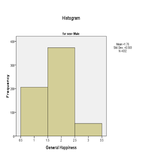
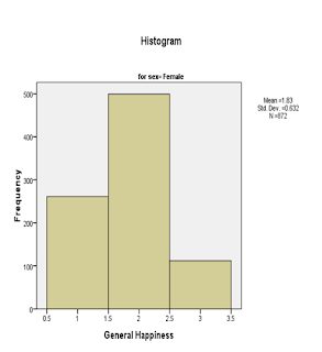
1. Have a look at the Histogram and check the tails of distribution if there are data points falling away as the extremes.
2. Inspect the Boxplot whether SPSS identifies outliers. These outliers are displayed as little circles with a ID number attached.
3. Make sure that the outlier's score is genuine and not an error.
4. Descriptive table provide you with an indication of how much a problem associated with these outlying cases. The expected value is the 5% Trimmed Mean. SPSS removes the top and bottom 5 per cent of the cases and calculated a new mean value to obtain this Trimmed Mean value. If you compare the original mean and this new trimmed mean, you can see if your more extreme scores are having a lot of influence on the mean. If you find these two mean values are very different, you need to investigate the data points further.
5. The Extreme values table gives you with the highest and the lowest values recorded for that variable and also provide the ID of the person with that score. It helps to identify the case that has the outlying values. SPSS Survival Manual by Julie Pallant

Read more...

Assessing the Normality of your Data

Many statistical analysis techniques hold the assumption that the distribution of scores on the dependent variable is normal. Normality is described as a symmetrical bell-shaped curve where the greatest frequency of the scores in the middle and with the smaller frequencies toward the extremes. Apart from checking normality of the skewness and kurtosis values, using the Explore option of the Descriptive Statistics menu is another way of doing it.

Procedure for Assessing Normality Using Explore

1. From the menu at the top of the screen click on Analyze, then click on Descriptive Statistics, then Explore.
2. Click on the variable/s you are interested in (e.g. total perceived stress). Click on the arrow button to move them in the Dependent List box.
3. Click on any independent or grouping variables that you wish to split your sample by (e.g. sex).
4. In the Display section make sure that Both is selected. This displays both the plots and statistics generated.
5. Click on the Plots button. Under Descriptive click on the Histogram. Click on Normality plots with tests.
6. Click on Continue.
7. Click on the Options button. In the Missing Values section click on Exclude cases pairwise.
8. Click on Continue and then OK.

The output generated from this procedure is shown below.

In the table labeled Descriptives, you are provided with descriptive statistics and other information concerning your variables. In the Test of Normality table above, you are provided with the results of the Kolmogorov-Smirnov statistic. This assesses the normality of the distribution of scores. A non-significant result (Sig value of more than .05) indicates normality. In this case, the Sig. Value is .000 for each group suggests violation of the assumption of normality.

Read more...

Obtaining Descriptive Statistics for Continous Variables

We have talked about the procedure to obtain descriptive statistics for categorical variables. Now, I want to show you the procedure of obtaining descriptive statistics for continuous variables:

1. From the menu at the top of the screen, click on Analyze, then click on Descriptive Statistics, then Descriptives.
2. Click on all the continuous variables that you want to obtain descriptive statistics for. Click on the arrow button to move them into the variable box (e.g., age).
3. Click on the Options button. Click on mean, standard deviation, minimum, maximum, skewness, kurtosis.
4. Click on Continue, and then OK.

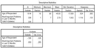
The output generated:

Reading the output:

Regarding the variable age, we have information from 1514 respondents, the range of ages is from 18 to 82 years, with a mean of 45.63 and standard deviation of 17.81 This information might be needed to be included in the method section of a research report to describe the characteristics of the sample.

The skewness value indicates that symmetry of the distribution. Kurtosis on the other hand provides information about the peakedness of the distribution. The value of 0 for skewness and kurtosis will be obtained when the distribution is perfectly normal. While positive skewness value indicates that the scores clustered to the left at the low values, negative skewness value indicates that scores clustered to the right-hand of the graph. While positive kurtosis value indicates that the distribution is rather peaked (clustered in the center) with long thin tails, the negative value indicates that a distribution is relatively flat due to the high number of extreme cases.

Read more...